Trading by Prediction
Contents
Trading by Prediction#
import numpy as np
import pandas as pd
from sklearn.preprocessing import LabelEncoder
import joblib
import matplotlib.pyplot as plt

# load our modules
import sys
sys.path.append("../../")
import lstm
import profit
Load Data#
We again consider the Tesla stock of the latest 90 days.
stocks: pd.DataFrame = pd.read_csv("../../data/stocks.csv", index_col=0, parse_dates=True)
company = "TSLA"
stock = stocks.query(f"Company == '{company}'").drop(columns=["Company", "Sector"])
num_days = 90
stock = stock[-num_days:]
stock
| Open | High | Low | Close | Volume | |
|---|---|---|---|---|---|
| Date | |||||
| 2022-06-27 | 249.366669 | 252.070007 | 242.566666 | 244.919998 | 89178300 |
| 2022-06-28 | 244.483337 | 249.970001 | 232.343338 | 232.663330 | 90391200 |
| 2022-06-29 | 230.500000 | 231.173340 | 222.273331 | 228.490005 | 82897200 |
| 2022-06-30 | 224.509995 | 229.456665 | 218.863327 | 224.473328 | 94600500 |
| 2022-07-01 | 227.000000 | 230.229996 | 222.119995 | 227.263336 | 74460300 |
| ... | ... | ... | ... | ... | ... |
| 2022-10-26 | 219.399994 | 230.600006 | 218.199997 | 224.639999 | 85012500 |
| 2022-10-27 | 229.770004 | 233.809998 | 222.850006 | 225.089996 | 61638800 |
| 2022-10-28 | 225.399994 | 228.860001 | 216.350006 | 228.520004 | 69152400 |
| 2022-10-31 | 226.190002 | 229.850006 | 221.940002 | 227.539993 | 61554300 |
| 2022-11-01 | 234.050003 | 237.399994 | 227.279999 | 227.820007 | 62566500 |
90 rows × 5 columns
Load Trained Model#
Recall that to use our PricePredictor, we need a feature encoder.
# set up feature encoder for the price predictor
feature_encoder = LabelEncoder()
feature_encoder.fit(lstm.ALL_FEATURES)
LabelEncoder()
Pass the encoder to the class attribute:
lstm.PricePredictor.feature_encoder = feature_encoder
Convert Pandas DataFrame to NumPy array:
# select the features of interest in data frame and transform it to NumPy array
stock = stock[lstm.ALL_FEATURES]
ts = stock[feature_encoder.classes_].to_numpy()
Load our trained model with joblib module:
Note
In fact, Scikit-Learn recommends to use joblib to load the models instead of pickle module.
price_predictor = joblib.load("../../models/TSLA-3-day-predictor.pkl")
price_predictor
PricePredictor(features=['Open', 'Volume', 'Close'], hidden_size=16,
               num_days_ago=400, pred_len=3, seq_len=30)
Information About the Stock Price of Future 1, 2 or 3 Days#
In this notebook, we choose to refer the predicted closing price the day after tomorrow. (num_days_ahead equals 2.)
num_days_ahead = 2
For each day, what the model does is that it takes into consideration all past days before the current day and predict the closing price N days from now. (N equals num_days_ahead. Since the model we have loaded can predict at most 3 days ahead, N can only be 1, 2 or 3.)
# use price predictor to predict future prices
sliding_prices = price_predictor.predict(ts)
future_prices = sliding_prices[1:, num_days_ahead-1]

# compare current and future closing prices
stock = stock.copy()[["Close"]]
stock["Future"] = future_prices

stock
| Close | Future | |
|---|---|---|
| Date | ||
| 2022-06-27 | 244.919998 | 245.929047 |
| 2022-06-28 | 232.663330 | 243.220215 |
| 2022-06-29 | 228.490005 | 237.126190 |
| 2022-06-30 | 224.473328 | 231.133057 |
| 2022-07-01 | 227.263336 | 229.120163 |
| ... | ... | ... |
| 2022-10-26 | 224.639999 | 219.918671 |
| 2022-10-27 | 225.089996 | 223.878922 |
| 2022-10-28 | 228.520004 | 226.528946 |
| 2022-10-31 | 227.539993 | 227.581192 |
| 2022-11-01 | 227.820007 | 229.530670 |
90 rows × 2 columns
Strategy#
The strategy is rather straight forward.
If the future price drops, and we are holding some shares, then we must sell all of it.
If the future price rises, and we don’t have any shares, then it is a good time to buy.
# Find buying and selling dates
buy_dates = []
sell_dates = []
is_holding_shares = False
for date, row in stock.iterrows():
    if is_holding_shares:
        # price will go down, sell it!
        if row["Future"] < row["Close"]:
            sell_dates.append(date)
            is_holding_shares = False
    else:
        # price will go up, buy!
        if row["Future"] > row["Close"]:
            buy_dates.append(date)
            is_holding_shares = True

# convert to Pandas `DatetimeIndex`
buy_dates = pd.DatetimeIndex(buy_dates)
sell_dates = pd.DatetimeIndex(sell_dates)

buy_dates, sell_dates
(DatetimeIndex(['2022-06-27', '2022-07-11', '2022-07-18', '2022-07-20',
                '2022-07-25', '2022-08-01', '2022-08-11', '2022-08-17',
                '2022-08-26', '2022-09-02', '2022-09-13', '2022-09-20',
                '2022-09-29', '2022-10-05', '2022-10-07', '2022-10-14',
                '2022-10-20', '2022-10-24', '2022-10-31'],
               dtype='datetime64[ns]', freq=None),
 DatetimeIndex(['2022-07-05', '2022-07-14', '2022-07-19', '2022-07-21',
                '2022-07-29', '2022-08-10', '2022-08-12', '2022-08-23',
                '2022-09-01', '2022-09-06', '2022-09-19', '2022-09-26',
                '2022-10-04', '2022-10-06', '2022-10-12', '2022-10-17',
                '2022-10-21', '2022-10-25'],
               dtype='datetime64[ns]', freq=None))
We now visualize the buying and selling dates:
# plot the last 90 days
plt.figure(figsize=(12, 4))
df = stock.copy()
df["Buy"] = np.nan
df.loc[buy_dates, "Buy"] = df.loc[buy_dates, "Close"]
df["Sell"] = np.nan
df.loc[sell_dates, "Sell"] = df.loc[sell_dates, "Close"]
plt.plot(df["Close"], label="Stock Price", color="k", alpha=0.5)
plt.scatter(
    df.index, df["Buy"],
    marker="^", color="r", zorder=2,
    label="Buy"
)
plt.scatter(
    df.index, df["Sell"],
    marker="v", color="g", zorder=2,
    label="Sell"
)
plt.legend()
plt.grid()
plt.show()
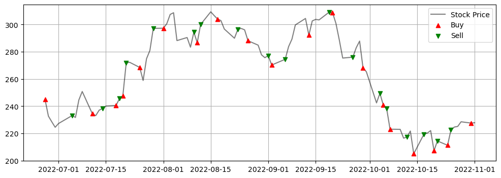
As we can see, this strategy suggests to trade more often than that of the moving average approach. And, it tends to seize every opportunity to increase the profit.
Profit#
Use the calc_profit function from our profit module to calculate the profit rate:
profit_rate = profit.calc_profit(
    stock,
    buy_dates, sell_dates,
    start_date="2022-06-27"
)

print(f"Profit rate: {100 * profit_rate:.2f}%")
Profit rate: 17.05%
Recall the profit rate with moving average strategy is 9.19%. Hence, the strategy proposed in this section is somewhat better.