Visualization

import pandas as pd
import matplotlib.pyplot as plt

Load Data

stocks = pd.read_csv("../../data/stocks.csv", index_col=0, parse_dates=True)
stocks

	Company	Sector	Open	High	Low	Close	Volume
Date
2017-11-02	AAPL	Technology	41.650002	42.125000	41.320000	42.027500	165573600
2017-11-03	AAPL	Technology	43.500000	43.564999	42.779999	43.125000	237594400
2017-11-06	AAPL	Technology	43.092499	43.747501	42.930000	43.562500	140105200
2017-11-07	AAPL	Technology	43.477501	43.812500	43.400002	43.702499	97446000
2017-11-08	AAPL	Technology	43.665001	44.060001	43.582500	44.060001	97638000
...	...	...	...	...	...	...	...
2022-10-26	COP	Energy	124.720001	128.179993	124.580002	126.570000	8139100
2022-10-27	COP	Energy	127.699997	129.449997	126.239998	126.639999	8948500
2022-10-28	COP	Energy	128.500000	128.990005	124.010002	127.169998	7293200
2022-10-31	COP	Energy	125.580002	129.990005	125.570000	126.089996	7121000
2022-11-01	COP	Energy	128.740005	129.320007	126.889999	127.779999	5874800

63377 rows × 7 columns

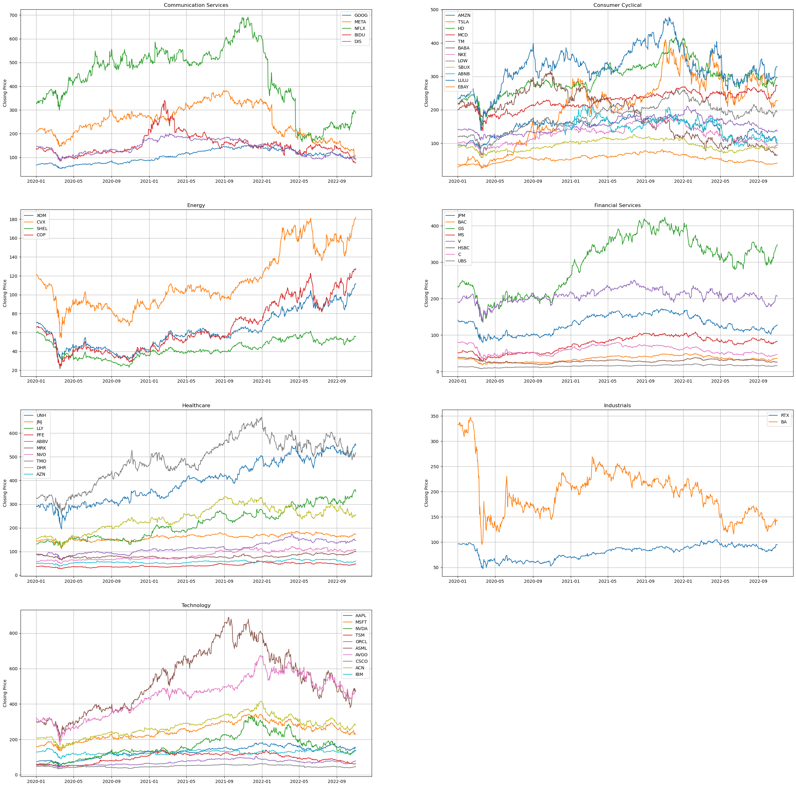
Trend of Closing Prices

sectors = stocks["Sector"].unique()
sectors.sort()
sectors

array(['Communication Services', 'Consumer Cyclical', 'Energy',
       'Financial Services', 'Healthcare', 'Industrials', 'Technology'],
      dtype=object)

Function to plot stocks in a given sector:

def plot_closing_price(sector: pd.DataFrame, ax: plt.Axes):
    
    df = stocks[stocks["Sector"] == sector]
    df = df[df.index >= "2020-01-01"]

    for company in df["Company"].unique():
        closing_price = df[df["Company"] == company]["Close"]
        ax.plot(closing_price, label=company)
    
    ax.set_title(sector)
    ax.set_ylabel("Closing Price")
    ax.legend()
    ax.grid()

Plot all sectors:

fig, axs = plt.subplots(4, 2, figsize=(32, 32))
axs = axs.flatten()

for i in range(7):
    plot_closing_price(sectors[i], axs[i])

# delete the last empty axes
plt.delaxes(axs[7])
plt.show()

Evaluate Companies by Dollar Volumes

The Dollar Volume can be computed by

\[ \text{Dollar Volume} = \text{Closing Price} \times \text{Volume} \]

Find the company with maximum average dollar volume in each sector:

df = stocks.copy()
df["Dollar Volume"] = stocks["Close"] * stocks["Volume"]
df.groupby(["Company", "Sector"]).mean()\
    .sort_values("Dollar Volume", ascending=False)\
    .reset_index(level=(0, 1))\
    .drop_duplicates(["Sector"])\
    .set_index("Sector").sort_index()\
    .drop(columns=["Open", "High", "Low"])

	Company	Close	Volume	Dollar Volume
Sector
Communication Services	META	220.069316	2.337455e+07	4.929304e+09
Consumer Cyclical	TSLA	126.995117	1.317317e+08	1.306260e+10
Energy	XOM	68.636971	2.044632e+07	1.327712e+09
Financial Services	BAC	32.406224	5.806661e+07	1.825491e+09
Healthcare	UNH	332.375851	3.532888e+06	1.128240e+09
Industrials	BA	262.674833	1.174971e+07	2.541470e+09
Technology	AAPL	94.923971	1.178255e+08	1.039713e+10