Effective Portfolio

import numpy as np
import pandas as pd
import json
import matplotlib.pyplot as plt

Candidate Companies

Recall that we have selected the most profitable company in each sector in the sense of dollar values. We now load the tickers of these candidate companies.

with open("../../data/companies.json", "r") as f:
    companies: list[str] = json.load(f)

companies

['META', 'TSLA', 'XOM', 'BAC', 'UNH', 'BA', 'AAPL']

We then put the closing prices of these companies side by side in a data frame:

num_days = 90

# load data
stocks: pd.DataFrame = pd.read_csv("../../data/stocks.csv", index_col=0, parse_dates=True)

df_list = []
for company in companies:
    df = stocks.query(f"Company == '{company}'")[["Close"]]
    df.rename(columns={"Close": company}, inplace=True)
    df_list.append(df)

# join stock prices of different companies
df = pd.DataFrame.join(df_list[0], df_list[1:])

# leave last 90 days out
df = df[:-num_days]

df

	META	TSLA	XOM	BAC	UNH	BA	AAPL
Date
2017-11-02	178.919998	19.950666	83.529999	27.870001	211.100006	262.630005	42.027500
2017-11-03	178.919998	20.406000	83.180000	27.820000	212.869995	261.750000	43.125000
2017-11-06	180.169998	20.185333	83.750000	27.750000	212.119995	264.070007	43.562500
2017-11-07	180.250000	20.403334	83.580002	27.180000	212.699997	266.130005	43.702499
2017-11-08	179.559998	20.292667	83.470001	26.790001	210.770004	265.570007	44.060001
...	...	...	...	...	...	...	...
2022-06-17	163.740005	216.759995	86.120003	31.920000	452.059998	136.800003	131.559998
2022-06-21	157.050003	237.036667	91.480003	32.849998	480.320007	136.750000	135.869995
2022-06-22	155.850006	236.086670	87.860001	32.599998	489.679993	137.160004	135.350006
2022-06-23	158.750000	235.070007	85.209999	32.080002	499.809998	133.970001	138.270004
2022-06-24	170.160004	245.706665	86.900002	32.310001	495.640015	141.529999	141.660004

1168 rows × 7 columns

Stock Returns

A stock return is the change in price of an asset, investment, or project over time, which may be represented in terms of price change or percentage change. In fact, we have already introduced this concept when calculating the profit in a previous section.

\[ \text{Today's Stock Return} = \frac{\text{Today's Price} - \text{Yesterday's Price}}{\text{Yesterday's Price}} \]

Sometimes, it is preferred to use the log return:

\[ \text{Log Return} = \log \left( 1 + \text{Stock Return} \right) \]

# standard returns
stock_returns = df.pct_change().dropna()

# log returns
stock_returns = stock_returns.apply(lambda x : np.log(1 + x), axis=1)

stock_returns

	META	TSLA	XOM	BAC	UNH	BA	AAPL
Date
2017-11-03	0.000000	0.022566	-0.004199	-0.001796	0.008350	-0.003356	0.025779
2017-11-06	0.006962	-0.010873	0.006829	-0.002519	-0.003529	0.008824	0.010094
2017-11-07	0.000444	0.010742	-0.002032	-0.020754	0.002731	0.007771	0.003209
2017-11-08	-0.003835	-0.005439	-0.001317	-0.014453	-0.009115	-0.002106	0.008147
2017-11-09	-0.001449	-0.004610	0.005972	-0.011261	0.003741	-0.010866	-0.002045
...	...	...	...	...	...	...	...
2022-06-17	0.017683	0.017029	-0.059394	0.002195	-0.008875	0.025468	0.011467
2022-06-21	-0.041716	0.089424	0.060379	0.028719	0.060638	-0.000366	0.032236
2022-06-22	-0.007670	-0.004016	-0.040376	-0.007639	0.019300	0.002994	-0.003834
2022-06-23	0.018437	-0.004316	-0.030626	-0.016079	0.020476	-0.023532	0.021344
2022-06-24	0.069409	0.044255	0.019639	0.007144	-0.008378	0.054896	0.024222

1167 rows × 7 columns

Volatility

Suppose the proportion / weight of money we want to invest in each stock is \(w_i\). Then the volatility of the portfolio is given by

\[ \text{Volatility} = \sqrt{\mathbf{w}^\top \Sigma \mathbf{w}} \]

where \(\mathbf{w} = (w_1, \ldots, w_n)^\top\) (assuming there are \(n\) companies), and \(\Sigma\) is the covariance matrix of the daily stock returns, which can be computed by np.cov(stock_returns.T) or stock_returns.cov() since stock_returns is a DataFrame.

Covariance matrix of stock returns, \(\Sigma\):

Tip

It is recommended to use Pandas’ functions when experimenting if your data is a DataFrame since the output is somewhat nicer. While in actual production, NumPy is preferred.

stock_returns.cov()

	META	TSLA	XOM	BAC	UNH	BA	AAPL
META	0.000664	0.000371	0.000139	0.000207	0.000169	0.000284	0.000311
TSLA	0.000371	0.001678	0.000181	0.000260	0.000193	0.000457	0.000396
XOM	0.000139	0.000181	0.000449	0.000303	0.000172	0.000371	0.000154
BAC	0.000207	0.000260	0.000303	0.000500	0.000216	0.000436	0.000217
UNH	0.000169	0.000193	0.000172	0.000216	0.000362	0.000254	0.000198
BA	0.000284	0.000457	0.000371	0.000436	0.000254	0.001041	0.000295
AAPL	0.000311	0.000396	0.000154	0.000217	0.000198	0.000295	0.000429

Then, the volatility can be calculated by (assuming the weights are all equal)

num_companies = len(companies)

# assign equal weights
weight = np.ones(num_companies) / num_companies

# convert to column vector
weight_vec = weight.reshape((-1, 1))

# volatility
volatility = np.sqrt(weight_vec.T @ np.cov(stock_returns.T) @ weight_vec)
volatility = volatility.item()
volatility

0.01823466003794474

def calc_volatility(stock_returns: pd.DataFrame, weight: np.ndarray) -> float:
    
    # scale weights
    weight = weight / weight.sum()
    
    # convert to column vector
    weight_vec = weight.reshape((-1, 1))
    
    # volatility
    volatility = np.sqrt(weight_vec.T @ np.cov(stock_returns.T) @ weight_vec)
    volatility = volatility.item()
    
    return volatility

Weighted Stock Returns

For a certain portfolio, the weighted stock return is simply the sum of weighted returns of all invested stocks.

\[ \text{Weighted Stock Return} = \mathbf{w}^\top \mathbf{r} = \sum_{i=1}^n w_i r_i \]

where \(r_i\) is the average stock return of the \(i\)-th company.

weighted_stock_return = np.dot(weight, stock_returns.mean().to_numpy())
weighted_stock_return

0.0005017068811196133

def calc_weighted_stock_return(stock_returns: pd.DataFrame, weight: np.ndarray) -> float:
    
    # scale weights
    weight = weight / weight.sum()
    
    return np.dot(weight, stock_returns.mean().to_numpy())

Monte Carlo Simulation

We generate weight for each company is selected with equal probabilities and then calculate the stock return as well as the volatility.

# set seed
SEED = 7008
rng = np.random.RandomState(SEED)

# the weight for each company is selected with equal probabilities
m = 5000
simulated_weights = rng.random((m, num_companies))

from functools import partial

# calculate volatility for each portfolio
volatilities = np.apply_along_axis(
    partial(calc_volatility, stock_returns),
    axis=1,
    arr=simulated_weights
)

# calculate stock return for each portfolio
weighted_stock_returns = np.apply_along_axis(
    partial(calc_weighted_stock_return, stock_returns),
    axis=1,
    arr=simulated_weights
)

Plot the stock return against the volatility for each portfolio:

plt.scatter(volatilities, weighted_stock_returns, s=1)
plt.xlabel("Volatility")
plt.ylabel("Weighted Stock Return")
plt.grid()
plt.show()

Sharpe Ratio

The Sharpe ratio is given by

\[ \text{Shape Ratio} = \frac{\text{Stock Return}}{\text{Volatility}} \]

We want the portfolio with as high Sharpe ratio as possible since we prefer high stock return and low volatility.

# calculate Sharpe ratio
sharpe_ratio = weighted_stock_returns / volatilities

# find the portfolio that maximize the sharpe ratio
optimal_weight_ix = np.argmax(sharpe_ratio)
optimal_weight: np.ndarray = simulated_weights[optimal_weight_ix]

# scale the weights
optimal_weight = optimal_weight / optimal_weight.sum()

optimal_weight

array([0.00808913, 0.20070573, 0.10093622, 0.00323051, 0.34447254,
       0.01460107, 0.32796482])

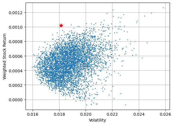
The optimal portfolio is marked as red star in the following plot:

plt.scatter(volatilities, weighted_stock_returns, s=1)
plt.scatter(volatilities[optimal_weight_ix], weighted_stock_returns[optimal_weight_ix], s=100, marker="*", color="r")
plt.xlabel("Volatility")
plt.ylabel("Weighted Stock Return")
plt.grid()
plt.show()