1.6. Shortest Paths and Dijkstra’s Algorithm

With every edge \(e\) in graph \(G\), we can associate a real number \(w(e)\), usually positive, which we shall call the weight of that edge. As we will see, to unify our notations for some special cases, it is convenient to define the weight of a nonexistent edge between two non-incident vertices as infinity \(\infty\).

We can now extend our former definition of the length of a path by

\[\begin{align*}\abs{P} := \sum_{e \in P} w(e) \end{align*}\]

Note that if all the edges are assigned to unit weights, then \(\abs{P}\) is just the number of edges in it, which reduces to the former definition. Notice also that the length of a trivial path is also zero since the sum of nothing in the above equation, by convention, is zero.

Given a map, the cities can be regarded as vertices, and for each pair of adjacent cities, we can draw an edge in between them. In this example, it is reasonable to define the weight of edge \(uv\) as the distance between cities \(u\) and \(v\). Then the problem of finding a shortest path from \(u_0\) to \(v\) arises quite naturally if we want to travel from city \(u_0\)(where we live) to every other city \(v\) at the minimum cost.

Formally, for all \(u, v \in V\), the length of the shortest path from \(u\) to \(v\) is defined as

\[\begin{split}\begin{align*} d(u,v) := \begin{cases} \min \set{\abs{P}}{\text{$P$ is a $(u, v)$-path}} , &\text{if $u$ and $v$ are connected} \\ \infty, &\text{if $u$ and $v$ are disconnected} \end{cases}\end{align*}\end{split}\]

Given a proper subset \(S\) of \(V\) and a source \(u_0 \in S\) in it, it is natural to define the distance from \(u_0\) to the complement \(S^\complement\) as the minimum distance from \(u_0\) to every \(v \in S^\complement\), that is,

\[\begin{align*} d(u_0, S^\complement) := \min_{v \in S^\complement} d(u_0, v) \end{align*}\]

Of course, if \(d(u_0, S^\complement) = \infty\), then there are no paths from \(u_0\) to any vertex in \(S^\complement\), in other words, \(u_0\) is disconnected from \(S^\complement\). Suppose \(d(u_0, S^\complement)\) is a finite number, which means there exists a path \(P = u_0 \cdots u v\) from \(u_0\) to some vertex \(v \in S^\complement\). The following are some simple observations about this path \(P\):

• ➀ \(P\) is a shortest \((u_0, v)\)-path,

• ➁ \(u \in S\) and the \((u_0, u)\)-section, \(u_0 \cdots u\), is a shortest \((u_0, u)\)-path, and

• ➂ we have the equation

(1.6)\[\begin{align} d(u_0, S^\complement) = d(u_0, u) + w(uv) \end{align}\]

Equation (1.6) motivates us to state the following proposition, which is the central idea of Dijkstra’s algorithm.

Proposition 1.12

Let \(G = (V, E)\) be a simple graph. Let \(S \subseteq V\) be a subset of vertices and \(u_0 \in S\) a point in it. We have

(1.7)\[\begin{align} d(u_0, S^\complement) = \min_{u \in S, v \in S^\complement}\{ d(u_0, u) + w(u v) \}\end{align}\]

Proof. First, note that the set

\[\begin{align*}\set{d(u_0, u) + w(u v)}{u \in S, v \in S^\complement}\end{align*}\]

is a finite set (possibly containing infinite numbers). Hence, it does have a minimum.

Assume there exist \(u^\ast \in S\) and \(v^\ast \in S^\complement\) such that

(1.8)\[\begin{align} d(u_0, S^\complement) > d(u_0, u^\ast) + w(u^\ast v^\ast) \end{align}\]

Note

Note that (1.8) implicitly implies that \(u_0\) and \(u^\ast\) are connected and \(u^\ast\) and \(v^\ast\) are connected since the right-hand side of (1.8) is a finite number.

Then there exists a \((u_0, u^\ast)\)-path \(P\) such that \(\abs{P} = d(u_0, u^\ast)\). Note that \(P v^\ast\) forms a path since all vertices in \(P\) are in \(S\) while \(v^\ast\) is in the complement \(S^\ast\). But \(P v^\ast\) is a path from \(u_0\) to \(S^\complement\) with length \(d(u_0, u^\ast) + w(u^\ast v^\ast)\), which is less than \(d(u_0, S^\complement)\) by assumption. Therefore, this leads to a contradiction. We have

\[\begin{align*} d(u_0, S^\complement) \leq d(u_0, u) + w(u v) \quad\forall u \in S \;\forall v \in S^\complement\end{align*}\]

And (1.7) is proved.

1.6.1. A First Attempt

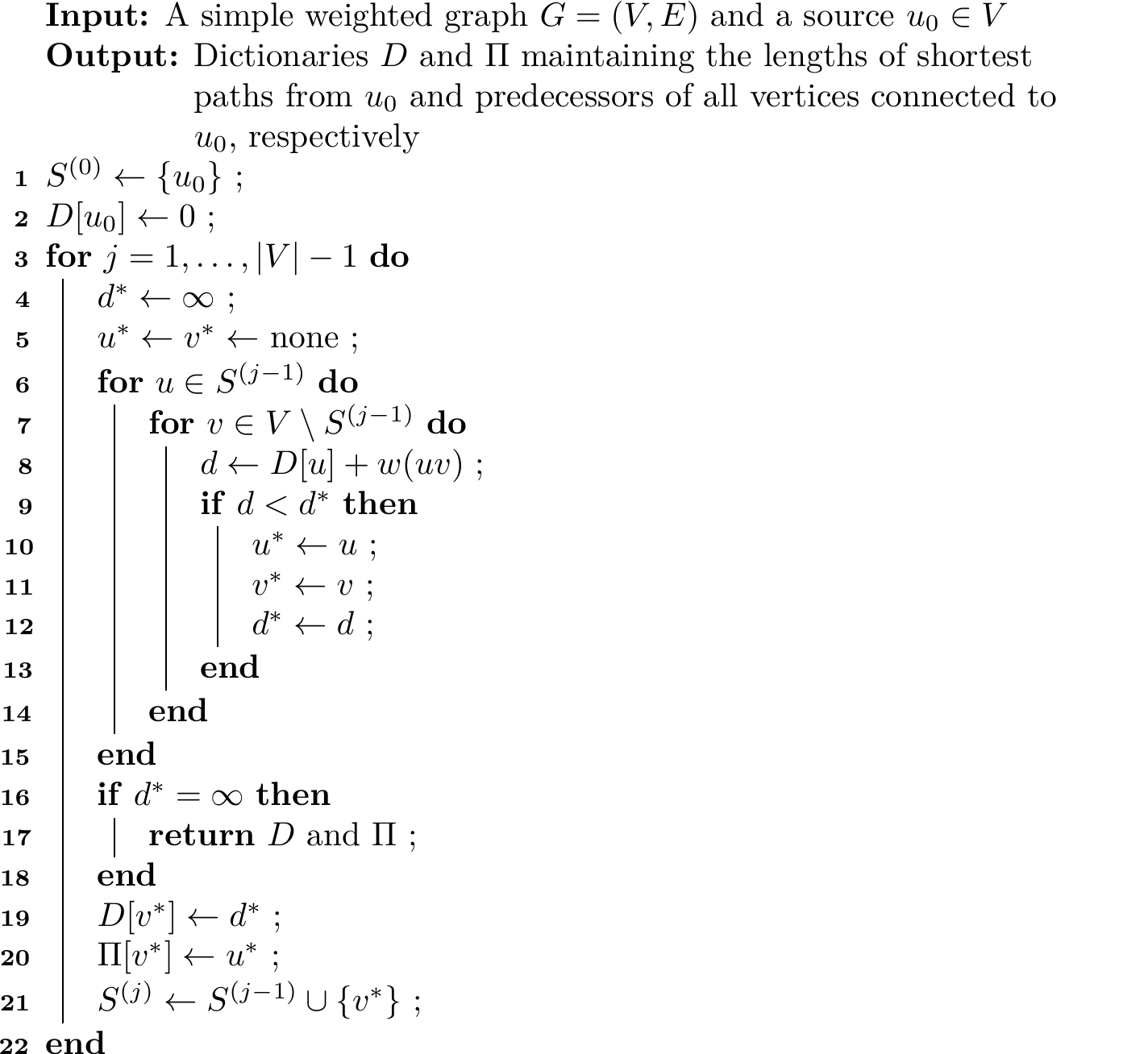
Starting from an initial set \(S^{(0)} = \{u_0\}\) containing just the source, we want to enlarge this set in a way that a shortest path from \(u_0\) to any vertex within the set is known. Given \(S^{(j-1)}\), in each iteration \(j\), we find optimal vertices \(u^\ast \in S^{(j-1)}\) and \(v^\ast \in V \setminus S^{(j-1)}\) in the sense that equation (1.7) is satisfied. In doing so, we are guaranteed to find a shortest path from \(u_0\) to \(V \setminus S^{(j-1)}\) with the terminus \(v^\ast\). Then we extend the set \(S^{(j-1)}\) to \(S^{(j)}\) by adding \(v^\ast\).

Based on this idea, we propose our first attempt to find shortest paths in the following algorithm (Algorithm 1.4).

Algorithm 1.4 (A First Attempt to Find the Shortest Paths)

1.6.2. Dijkstra’s Algorithm

Algorithm 1.5 (Dijkstra’s Algorithm)

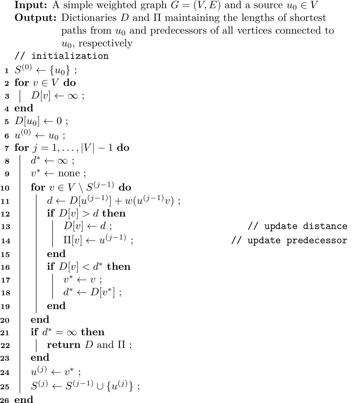
Given a vertex \(v\), its predecessor is given by \(\Pi[v]\). And the predecessor of \(\Pi[v]\) is \(\Pi[ \Pi[v] ]\), and so forth. We can keep accessing the predecessors until hopefully stops at the source \(u_0\). In this case, we have recovered a path from \(u_0\) to \(v\), \(u_0 \cdots \Pi[v] v\). To make our proof concise, we call this procedure recovering a \((u_0, v)\)-path using \(\Pi\).

Proof. Note that there is an early return in line 22. Hence, we may not complete all \(n-1\) iterations of the for loop (lines 7-23). Suppose we can complete \(k\) iterations.

Loop Invariants: Upon completion of the \(j\)-th iteration, we claim that

• ➀ \(D[u] = d(u_0, u) \quad \forall u \in S^{(j)}\),

• ➁ \(D[v] = \min_{u \in S^{(j-1)}} \{ d(u_0, u) + w(u v) \} \quad \forall v \in V \setminus S^{(j)}\),

• ➂ we can recover a \((u_0, u)\)-path using \(\Pi\) for every \(u \in S^{(j)}\), and

• ➃ \(S^{(j)} = S^{(j-1)} \uplus u^{(j)}\).

Maintenance: Assuming all loop invariants hold for \(j-1\). We now consider the \(j\)-th iteration. In the inner loop (lines 10-20), by referring to loop invariant 2, we note that the procedure from line 11 to line 15 ensures that

(1.9)\[\begin{align} D[v] = \min\left\{\min_{u \in S^{(j-2)}}\{ d(u_0, u) + w(u v) \}, D[u^{(j-1)}] + w(u^{(j-1)} v) \right\}\quad\forall v \in V \setminus S^{(j-1)}\end{align}\]

after this inner loop is completed. But invariant 1 implies that \(D[u^{(j-1)}] = d(u_0, u^{(j-1)})\). Moreover, we have \(S^{(j-1)} = S^{(j-2)} \uplus u^{(j-1)}\) by invariant 4. Hence, (1.9) reduces to

(1.10)\[\begin{split}\begin{multline} D[v] = \min\left\{\min_{u \in S^{(j-2)}}\{ d(u_0, u) + w(u v) \}, d(u_0, u^{(j-1)}) + w(u^{(j-1)} v) \right\}\\ = \min_{u \in S^{(j-1)}}\{ d(u_0, u) + w(u v) \}\quad\forall v \in V \setminus S^{(j-1)}\end{multline}\end{split}\]

Note that invariant 2 for iteration \(j\) follows directly from (1.10) because \(V \setminus S^{(j)} \subseteq V \setminus S^{(j-1)}\) by line 25 if line 25 is reachable in the current iteration. If line 25 is not reachable, which means the algorithm terminates at line 22, then there is nothing to prove for this iteration.

The purpose of lines 16-19 is that upon completion of lines 10-20, we have

\[\begin{align*} d^\ast = \min_{v \in V \setminus S^{(j-1)}}\min_{u \in S^{(j-1)}}\{ d(u_0, u) + w(u v) \}\end{align*}\]

By Proposition 1.12, we know \(d^\ast\) is the length of a shortest path from \(u_0\) to \(V \setminus S^{(j-1)}\), that is,

\[\begin{align*} d^\ast = d(u_0, V \setminus S^{(j-1)}) \end{align*}\]

We are now at the end of line 20. There are two cases.

(Case 1: Early Return) If \(d^\ast = \infty\) or equivalently \(d(u_0, V \setminus S^{(j-1)}) = \infty\), then it means that \(u_0\) is disconnected from \(V \setminus S^{(j-1)}\). Since no shortest paths are to be discovered, the algorithm needs to terminate. Recall we assume we can only complete \(k\) iterations. Therefore, the current iteration must be \(k+1\) for we are exiting the algorithm. No loop invariants need to be proved since this iteration is not completed.

(Case 2) On the other hand, we now suppose \(v^\ast\) is some vertex at the end of line 20. Let \(u^{(j)} = v^\ast\)(line 24). Then invariant 4 for iteration \(j\) is proved immediately by line 25.

We now prove invariant 3 for \(j\). Note that the predecessor of \(u^{(j)}\) is \(u^{(j-1)}\), i.e., \(\Pi[u^{(j)}] = u^{(j-1)}\) by line 14. We then recover a \((u_0, u^{(j-1)})\)-path, say \(P\), using \(\Pi\)(invariant 3 for \(j-1\)). Note that \(P u^{(j)}\) is a \((u_0, u^{(j)})\)-path, and it can be recovered using \(\Pi\) since \(\Pi[u^{(j)}] = u^{(j-1)}\) and \(P\) itself is recovered using \(\Pi\). This proves invariant 3 of iteration \(j\).

Furthermore, by recalling \(u^{(j)} = v^\ast\) and \(d^\ast = d(u_0, V \setminus S^{(j-1)})\), we note that \(P u^{(j)}\) is a shortest path from \(u_0\) to \(u^{(j)}\) since its length is \(d(u_0, V \setminus S^{(j-1)})\). In other words, it is also a shortest path from \(u_0\) to \(V \setminus S^{(j-1)}\). Therefore, we can write

\[\begin{align*} d(u_0, u^{(j)}) = d^\ast = D[v^\ast]\end{align*}\]

where the last equality follows from line 18. Replacing \(v^\ast\) with \(u^{(j)}\), equivalently we have

(1.11)\[\begin{align} D[u^{(j)}] = d(u_0, u^{(j)}) \end{align}\]

This equation (1.11) along with invariant 1 for \(j-1\) implies that invariant 1 also holds for \(j\). Note that we have shown that all loop invariants are preserved when the current iteration (iteration \(j\)) is completed.

Termination: As the algorithm terminates, there are \(k+1\) vertices in \(S^{(k)}\). And the vertices outside \(S^{(k)}\) are not reachable from the source \(u_0\). For each \(u \in S^{(k)}\), we have \(D[u] = d(u_0, u)\)(invariant 1), that is, \(D[u]\) stores the length of a shortest path from \(u_0\) to \(u\), as desired. And by invariant 3, we can recover a shortest \((u_0, u)\)-path using \(\Pi\). This completes the proof.