1.3. Graph Realization Problem

Let \(G\) be a graph with vertices \(v_1, \ldots, v_n\). The degree sequence of \(G\), as the name suggests, is a list of integers consists of vertex degrees. It is denoted by

\[\begin{align*}\mathbf{d} = (\deg(v_1), \ldots, \deg(v_n)) \end{align*}\]

And it is often written in decreasing order.

Given an arbitrary list of non-negative integers \(\mathbf{d}^\prime = (d_1^\prime, \ldots, d_n^\prime)\), it is possible that we cannot find any graphs whose degree sequence is \(\mathbf{d}^\prime\). For example, no graphs have the following degree sequence:

\[\begin{align*}(2, 2, 1, 1, 1) \end{align*}\]

Why? Note that \(2+2+2+1+1+1 = 9\). Hence, by Theorem 1.1, we see that is is impossible to find such a graph since the sum of degrees should be an even number. Alternatively, one may also argue by Corollary 1.1 that the number of odd vertices (the last three vertices) is 3, which is an odd number.

So, what conditions must a list of non-negative integers must satisfy so that it is a degree sequence? The answer is simple, as the next proposition will show, the provided list of integers only need to satisfy condition given in Theorem 1.1, that is, all the integers need to sum up to an even number.

Proposition 1.3

A sequence \((d_1, \ldots, d_n)\) of non-negative integers is a degree sequence if and only if \(\sum_{i=1}^n d_i\) is even.

Proof. TODO

From the above proof, we see that the graph we construct is a multigraph since we mainly increase the vertex degrees by adding loops. This invites us to think can we construct a simple graph out of the given sequence of integers? This question is much more complecated. And we say that a sequence of integers is graphical if it is a degree sequence of some simple graph. The problem of finding such a simple graph is referred to as the graph realization problem.

1.3.1. Havel-Hakimi Theorem

The algorithm [Hakimi, 1962] constructs a simple graph through a recursive procedure. The theorem it based on is referred to as Havel-Hakimi theorem. Before proving this theorem, we first introduce a lemma, which will be helpful in the later proof.

Lemma 1.1

Let \(G\) be a simple graph. If

• ➀ \(u_1 v_1, u_2 v_2 \in E\) and

• ➁ \(u_1 v_2, u_2 v_1 \notin E\),

then all vertex degrees in the graph

\[\begin{align*} G^\prime = G - \{u_1 v_1, u_2 v_2\} + \{u_1 v_2, u_2 v_1\}\end{align*}\]

remain unchanged. Of course, \(G^\prime\) has the same degree sequence as \(G\).

This lemma mainly says we can move two non-incident edges in \(G\) in a way that the degree sequence remains unchanged. Refer to Fig. 1.2 to get more insight.

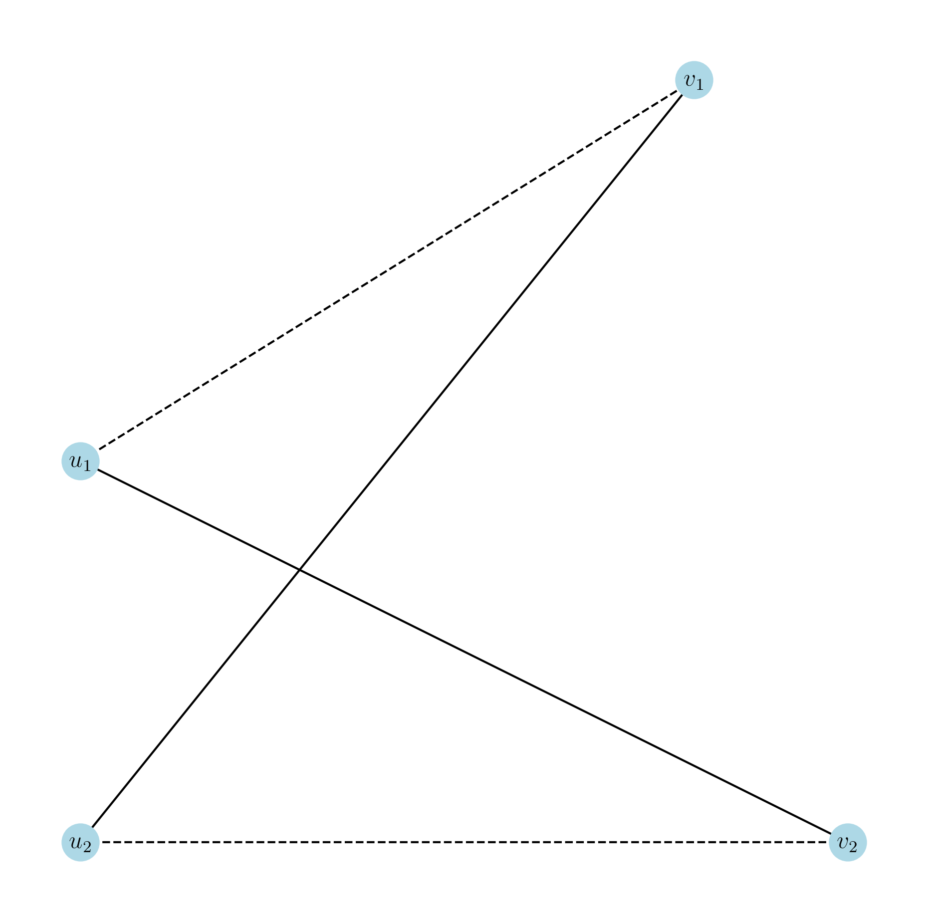
Fig. 1.2 Dash lines are removed edges while solid lines are newly added.

Proof. This result is evident. We note that the degrees of vertices \(u_1\), \(v_1\), \(u_2\) and \(v_2\) remain unchanged in \(G^\prime\) since from the perspective of each of these four vertices, one incident edge is removed but a new one is added. And the degrees of all the other vertices in \(G^\prime\) are also the same as in \(G\).

We now present the Havel-Hakimi theorem.

Theorem 1.2 (Havel-Hakimi)

Let \(\mathbf{d}=(d_1, \ldots, d_n)\) be a decreasing sequence of non-negative integers. Define \(\mathbf{d}^\prime\) as

\[\begin{align*}\mathbf{d}^\prime = ( \underbrace{ d_2 - 1, \ldots, d_{d_1 + 1} - 1 }_{\text{$d_1$ terms}}, d_{d_1 + 2}, \ldots, d_n ) \end{align*}\]

Then \(\mathbf{d}\) is graphical if and only if \(\mathbf{d}^\prime\) is graphical.

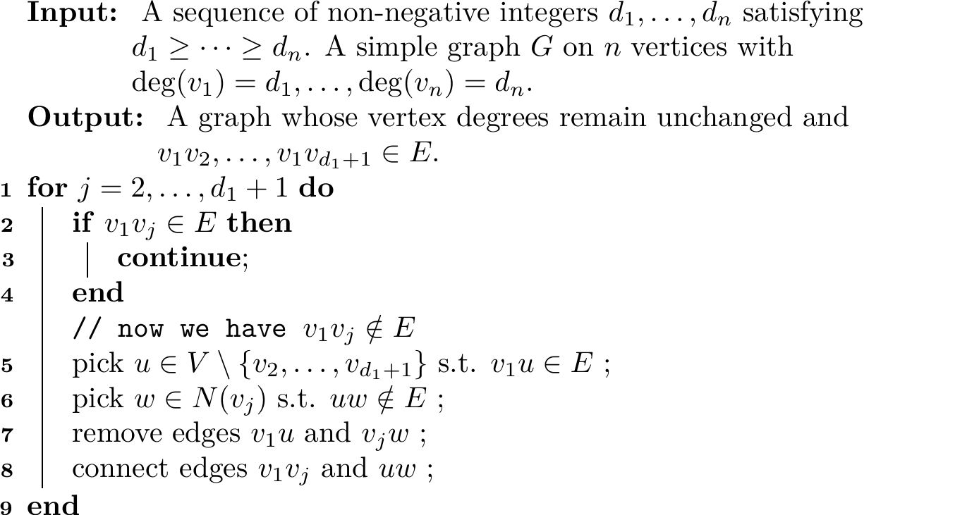
Algorithm 1.1 (Reconnecting Graph Edges in Proving Havel-Hakimi Theorem)

Proof. (\(\impliedby\)) Let \(G^\prime\) be a simple graph with degree sequence \(\mathbf{d}^\prime\). Suppose \(V(G^\prime) = v_2, \ldots, v_n\) and

\[\begin{align*}\deg(v_2) = d_2 - 1, \;\ldots, \;\deg(v_{d_1 + 1}) = d_{d_1 + 1} - 1, \;\deg(v_{d_1 + 2}) = d_{d_1 + 2}, \;\ldots, \;\deg(v_n) = d_n \end{align*}\]

Now, find a vertex, say \(v_1\), that is distinct from the existing vertices of \(G^\prime\), and then join \(v_1\) with \(v_2, \ldots, v_{d_1 + 1}\). We call the resulting graph \(G\). Observe that \(\deg(v_1) = d_1\) and the degrees of \(v_2, \ldots, v_{d_1 + 1}\) are all increased by one. Hence, the degree sequence of \(G\) is exactly \(\mathbf{d}\).

(\(\implies\)) Suppose that \(G\) is a graph with degree sequence \(\mathbf{d}\) and that

\[\begin{align*}\deg(v_1) = d_1, \;\ldots, \;\deg(v_n) = d_n \end{align*}\]

Note

The difficulty of proving this direction is that \(v_1\) is not necessarily to be incident with \(v_2, \ldots, v_{d_1 + 1}\). So, we need to design an algorithm to alter the original graph without changing its degree sequence so that \(v_1\) is incident with \(v_2, \ldots, v_{d_1 + 1}\). See Algorithm 1.1.

In the following, we prove the correctness of Algorithm 1.1.

Loop Invariants: Upon completion of iteration \(j\), we have

• ➀ All vertex degrees remain the same, and

• ➁ \(v_1 v_2, \ldots, v_1 v_j \in E\).

(Note that there is no need to prove the initialization part of this algorithm.)

Maintenance: If the condition in line 2 is satisfied, then the loop invariant holds. Now, suppose that \(v_1 v_j \notin E\).

We first show why line 5 works. Assume we cannot find such vertex \(u\), which means \(v_1\) is not incident with any vertex other than \(\{v_2, \ldots, v_{d_1 + 1}\}\). Because \(v_1\) is incident with \(d_1\) vertices, it must be incident with all vertices in \(\{v_2, \ldots, v_{d_1 + 1}\}\), which leads to a contradiction since \(v_1 v_j \notin E\). Hence, we can always find such a \(u\) specified by line 5.

Let us now prove the correctness of line 6. Assume, on the contrary, there is no such vertex \(w\). Then \(u\) is incident with every neighbor of \(v_j\), which implies that

\[\begin{align*}\deg{u}\geq\deg(v_j) \end{align*}\]

Moreover, \(u\) is also incident with \(v_1\) whereas \(v_j\) is not. Hence,

\[\begin{align*}\deg{u} > \deg(v_j) \end{align*}\]

But the degree of \(u\) should be less than or equal to that of \(v_j\) based on the given condition. Hence, this leads to a contradiction and line 6 also works.

Since \(v_1 u, w v_j \in E\) and \(v_1 v_j, w u \notin E\), by applying Lemma 1.1, we know that all vertex degrees remain unchanged after executing line 7 and line 8. (Note that now \(v_1 v_j \in E\).) This proves the loop invariants.

Termination: Upon termination, the result is as desired due to the loop invariants.

Now, by removing vertex \(v_1\), we will reduce the degree of \(v_2, \ldots, v_{d_1 + 1}\) by one. Hence, \(G^\prime = G - v_1\) has the degree sequence \(\mathbf{d}^\prime\), and it is of course simple. Therefore, \(\mathbf{d}^\prime\) is graphical.